top of page

FOUNDRY-IN-A-BOX 4.0
CFD Casting Tutorial
1. Create Case
Open SimFlow and click on New. Create a name for your case simulation and click Create Case. If you want to open an existing case, click on Open and select a case from the list of optinos.

2. Import STL
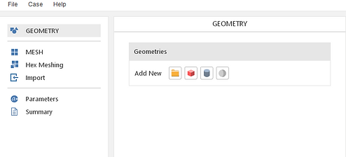
For this tutorial, we will be using the Tutorial Mold file. To open it into SimFlow, go to the Add New box and click on the folder icon. Then, open the file.
3. Adjust geometry
When importing in the STL file, the geometry will be too big. Click on the 3 dots next to the STL name and then click on Scale. A Scale Geometry window will then pop up. Make sure to check the box next to Uniform and add in a scaling factor of 0.001.


4. Mesh Geometry, Part 1
Now we need to create the mesh, or space, where our simulation will take place. Go to the Hex Meshing panel and enable meshing on the geometry by clicking where the blue square is.

5. Mesh Geometry, Part 2
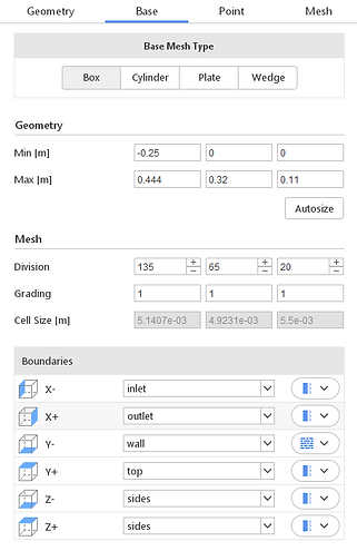
For Base Mesh Type, select Box. Then, plug in the minimum and maximum points as shown to the right. We will then divide our mesh so that the cell size is as close to 0.005 m as possible. It is possible to create a finer mesh, but please note that the version of SimFlow we are using only allows a maximum of 200k mesh blocks. For reference, this mesh has 83k mesh blocks.
Next, switch to the Base tab. Then, use the dropdown arrows to assign the following boundary conditions to each direction. To create the "sides" boundary condition, double click on the default boundary conditions and type in "sides". Then, assign the boundary condition to the Z- and Z+ directions.
6. Mesh Geometry, Part 3
Click on the Point tab and plug in the following X,Y,Z values (-0.11, 0.12, 0.055). Alternatively, you can CTRL-click on the orange arrows and drag the point to an appropriate location. Make sure that the point is within our mesh block but not touching or inside our geometry.

7. Mesh Geometry, Part 4
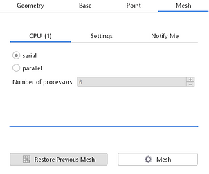
Finally, we can start the meshing process. Click on the Mesh tab and then click on the Mesh button. Leave all other default values. This may take a while, so please be patient.
8. Add 2nd Geometry
In this simulation, we will need a 2nd geometry for the simulation to work. Go back to the geometry tab and click on the red box icon. Add in the following values and rename the geometry name by double-clicking on box_1.

9. Select Solver
We will be using the InterFOAM solver for this simulation. Go to the available solvers list and scroll down until you see Inter. Or, click on Transient, Incompressible, and Multiphase in the filters list to find the Inter solver. Click on Inter and then click on Select. This will then unlock the tabs necessary to set up our simulation.

At this point, do not change the default settings of the tabs unless specified.
10. Transport Properties
The Transport Properties tab is where we assign the types of materials that will be used in the simulation. Double click on phase 1 and rename it to water. Then, while water is still selected, click on Material Database and scroll down to Water. Check the box next to Water and click Apply. If done correctly, your screen should like the image on the left.

11. Operating Conditions
In this tab, make sure to set a proper gravitational constant of -9.81 in the Y direction.

12. Boundary Conditions, Part 1
We will apply a volumetric flow rate in the inlet direction. Click on the inlet boundary and select Fixed Flux Pressure from the Type drop-down list. Then, select Variable Height Inlet and type in 0.0025.

13. Boundary Conditions, Part 2
Click on the Phases tab while in the Inlet boundary condition. Click on Zero Gradient for the type.

14. Boundary Conditions, Part 3
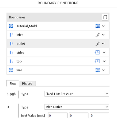
Click on the Outlet boundary. Just like the inlet, choose Fixed Flux Pressure, but leave the Type as Inlet-Outlet.
15. Boundary Conditions, Part 4
Click on the sides boundary and choose Zero Gradient and Slip.
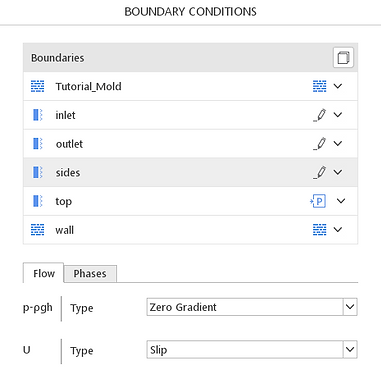
16. Boundary Conditions, Part 5
For the last boundary condition, click on the Phases tab for sides and choose Zero Gradient.
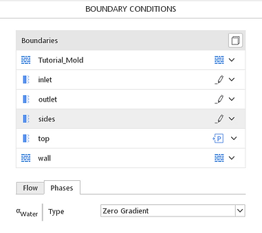
17. Initial Conditions
When we begin the simulation, we want our Initial_Volume geometry to already be water. Choose the alpha water field and make sure to check the box next to it. Then, assign a value of 1.
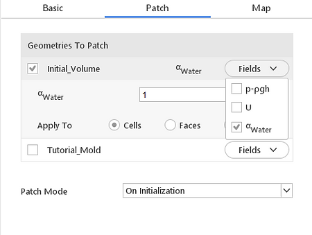
18. Monitors
Although we will do complete post-processing using Paraview, we can see the 3D model throughout the simulation using Monitors. Select the Sampling tab in Monitors and choose slice. We want an X-Y view of the entire mesh, so make the slice normal to the Z direction by assigning the values 0 0 1. Then, to translate the slice halfway across the mesh, give it the point 0 0 0.055. Make sure to check the boxes next to U and alpha water so we can see the values in 3D
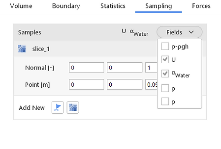
19. Run, Part 1
We will make our entire simulation time 5 seconds. Change Time Stepping to Automatic and include an initial time step of 0.01 seconds.

20. Run, Part 2
For Interval (s), type a value of 0.1. Therefore, our simulation will have a sampling rate of 0.1 seconds. Throughout our 5 second simulation, we will have data every 0.1 seconds. Finally, click on the Run button (Blue circle with white triangle) to start the simulation.

bottom of page